The Effects of Noise on Gamma

Here is an example of the effects noise can have on gamma. Simply by adding noise to the evaluation distribution the Gamma goes from a passing rate of about 50% to about 99%. For a Monte Carlo planning system this dose distribution includes statistical noise potentially pushing the Gamma pass rate artificially higher than should that noise be absent.

import numpy as np
import matplotlib.pyplot as plt

!pip install pymedphys

import pymedphys

Requirement already satisfied: pymedphys in /home/docs/checkouts/readthedocs.org/user_builds/pymedphys/envs/latest/lib/python3.8/site-packages (0.40.0)

Requirement already satisfied: setuptools in /home/docs/checkouts/readthedocs.org/user_builds/pymedphys/envs/latest/lib/python3.8/site-packages (from pymedphys) (69.2.0)
Requirement already satisfied: tomlkit in /home/docs/checkouts/readthedocs.org/user_builds/pymedphys/envs/latest/lib/python3.8/site-packages (from pymedphys) (0.12.4)
Requirement already satisfied: typing-extensions in /home/docs/checkouts/readthedocs.org/user_builds/pymedphys/envs/latest/lib/python3.8/site-packages (from pymedphys) (4.10.0)

gamma_options = {
    'dose_percent_threshold': 3,
    'distance_mm_threshold': 3,
    'lower_percent_dose_cutoff': 20,
    'interp_fraction': 10,  # Should be 10 or more for more accurate results
    'max_gamma': 2,
    'random_subset': None,
    'local_gamma': True,
    'ram_available': 2**29,  # 1/2 GB
    'quiet': True
}

grid = 0.5
scale_factor = 1.035
noise = 0.01

xmin = -28
xmax = 28
ymin = -25
ymax = 25

extent = [xmin-grid/2, xmax+grid/2, ymin-grid/2, ymax+grid/2]

Defining an example dose reference

Here we are defining an idealised square field using an exponential function. We are also creating a coords variable which we will be passing to the pymedphys.gamma function.

x = np.arange(xmin, xmax + grid, grid)
y = np.arange(ymin, ymax + grid, grid)

coords = (y, x)

xx, yy = np.meshgrid(x, y)
dose_ref = np.exp(-((xx/15)**20 + (yy/15)**20))

plt.figure()
plt.title('Reference dose')

plt.imshow(
    dose_ref, clim=(0, 1.04), extent=extent)
plt.colorbar();

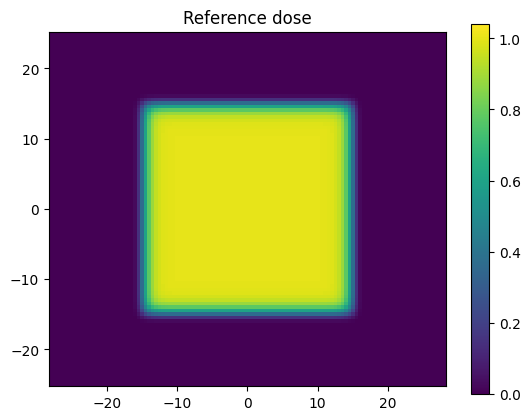
Of importance the length of the first coordinate set in coords matches the first dimension of dose_ref, and the length of the second coordinate set in coords matches the second dimension of dose_ref. This is required because pymedphys.gamma internally uses scipy.interpolate.RegularGridInterpolator and the gamma implimentation has been chosen to align with this scipy coordinate convention uses here.

len(coords[0])

101

len(coords[1])

113

np.shape(dose_ref)

(101, 113)

dimensions_of_dose_ref = np.shape(dose_ref)
assert dimensions_of_dose_ref[0] == len(coords[0])
assert dimensions_of_dose_ref[1] == len(coords[1])

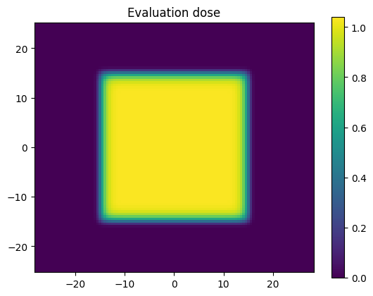
Defining an example evaluation dose

Let’s scale our reference dose by a scaling factor. We have chosen above to scale by 3.5% purposefully so that the dose will go larger than the dose percent evaluation criterion of 3% that was chosen above.

dose_eval = dose_ref * scale_factor

plt.figure()
plt.title('Evaluation dose')

plt.imshow(
    dose_eval, clim=(0, 1.04), extent=extent)
plt.colorbar();

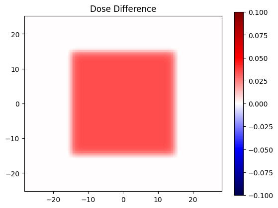
Seeing a dose difference

dose_diff = dose_eval - dose_ref

plt.figure()
plt.title('Dose Difference')

plt.imshow(
    dose_diff, 
    clim=(-0.1, 0.1), extent=extent,
    cmap='seismic'
)
plt.colorbar();

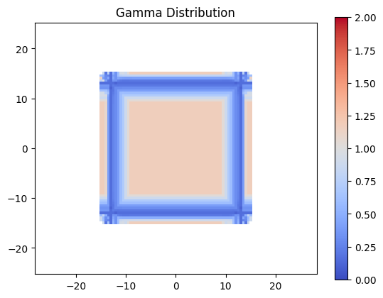
Evaluation Gamma

Now lets evaluate gamma for the distributions defined above. As expected, due to the dose being scaled larger than the dose threshold, quite a few points fail.

gamma_no_noise = pymedphys.gamma(
    coords, dose_ref,
    coords, dose_eval,
    **gamma_options)

plt.figure()
plt.title('Gamma Distribution')

plt.imshow(
    gamma_no_noise, clim=(0, 2), extent=extent,
    cmap='coolwarm')
plt.colorbar()

plt.show()
valid_gamma_no_noise = gamma_no_noise[~np.isnan(gamma_no_noise)]
no_noise_passing = 100 * np.round(np.sum(valid_gamma_no_noise <= 1) / len(valid_gamma_no_noise), 4)

plt.figure()
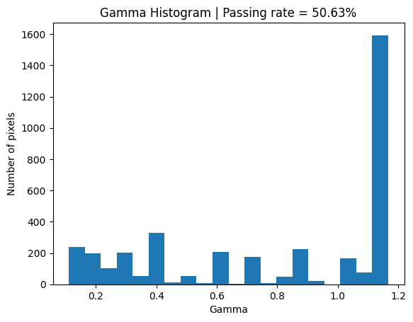
plt.title(f'Gamma Histogram | Passing rate = {round(no_noise_passing, 2)}%')
plt.xlabel('Gamma')
plt.ylabel('Number of pixels')

plt.hist(valid_gamma_no_noise, 20);

/tmp/ipykernel_697/3121033137.py:1: DeprecationWarning: Parameter `quiet` will be deprecated in the future
  gamma_no_noise = pymedphys.gamma(

Investigating the effect of noise

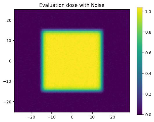
Let’s now slightly adjust our evaluation distribution by adding some random normal noise.

np.random.seed(0)
dose_eval_noise = (
    dose_eval + 
    np.random.normal(loc=0, scale=noise, size=np.shape(dose_eval))
)

plt.figure()
plt.title('Evaluation dose with Noise')

plt.imshow(
    dose_eval_noise, clim=(0, 1.04), extent=extent)
plt.colorbar();

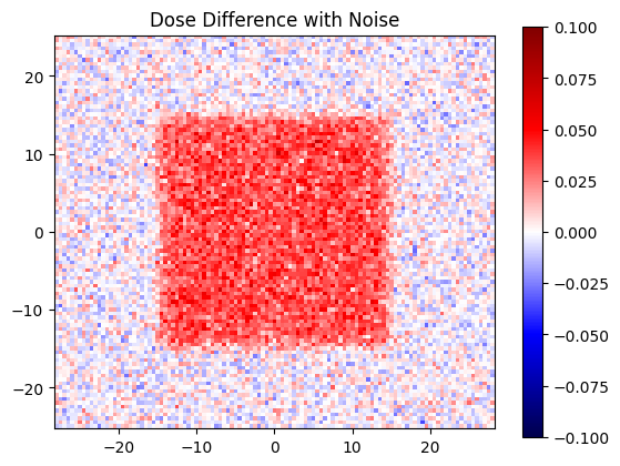
Let’s see what our dise difference looks like with this noise

dose_diff_with_noise = dose_eval_noise - dose_ref

plt.figure()
plt.title('Dose Difference with Noise')

plt.imshow(
    dose_diff_with_noise, 
    clim=(-0.1, 0.1), extent=extent,
    cmap='seismic'
)
plt.colorbar();

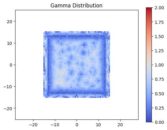
But what about our gamma?

gamma_with_noise = pymedphys.gamma(
    coords, dose_ref,
    coords, dose_eval_noise,
    **gamma_options)

plt.figure()
plt.title('Gamma Distribution')

plt.imshow(
    gamma_with_noise, clim=(0, 2), extent=extent,
    cmap='coolwarm')
plt.colorbar()

plt.show()
valid_gamma_with_noise = gamma_with_noise[~np.isnan(gamma_with_noise)]
with_noise_passing = 100 * np.round(np.sum(valid_gamma_with_noise <= 1) / len(valid_gamma_with_noise), 4)

plt.figure()
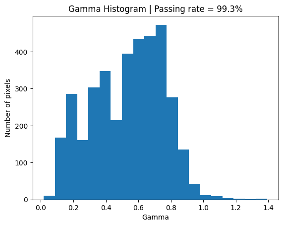
plt.title(f'Gamma Histogram | Passing rate = {round(with_noise_passing, 2)}%')
plt.xlabel('Gamma')
plt.ylabel('Number of pixels')

plt.hist(valid_gamma_with_noise, 20);

/tmp/ipykernel_697/511314066.py:1: DeprecationWarning: Parameter `quiet` will be deprecated in the future
  gamma_with_noise = pymedphys.gamma(

Conclusion

So, pymedphys does provide a gamma implementation, but should it be a defacto standard of validation? I highly recommend giving the following paper a read to highlight some other tools we can use to augment our usage of Gamma.

Evaluating IMRT and VMAT dose accuracy: Practical examples of failure to detect systematic errors when applying a commonly used metric and action levels

A key take home message from that paper relevant to this pymedphys.gamma utility is the following:

Using 3%G/3 mm gamma passing rates as a basis of gauging “sufficient accuracy” as per TG-119 has knock-on effects outside of commissioning. One such effect is that it is often used as the de facto standard to “validate” a new or modified product. For example, even very recently 3%G/3 mm passing rates have been quoted to prove the accuracy of TPS dose algorithms, delivery systems, or dosimetry devices.

In this work, we show a variety of clear examples of the metric’s insensitivity, supporting the argument that it is inappropriate as a sole basis for commissioning. The same conclusion can be made for the yet further upstream task of product validation by medical device manufacturers and their clinical partners.