Speeding up gamma calculations

The PyMedPhys gamma function allows the user to compute gamma ($\gamma$) index distributions between a reference and an evaluation dose distribution in 1D, 2D and 3D, and obtain gamma pass rates for these distributions.

In this tutorial, you will compute the gamma pass rate using the PyMedPhys gamma function. You will tweak its parameters to speed up the computation of the gamma index distribution.

You will test the PyMedPhys gamma on two 3D (and 2D) dose distributions, and you will focus on two of the PyMedPhys gamma parameters, max_gamma and random_subset, which are particularly useful when performing pass rate calculations.

First, we import the required modules and download the DICOM RTDOSE data that you will use

import pydicom
import pymedphys
import numpy as np

reference_filepath = pymedphys.data_path("original_dose_beam_4.dcm") # reference (e.g., calculated) dose
evaluation_filepath = pymedphys.data_path("logfile_dose_beam_4.dcm") # evaluation (e.g., measured) dose

Both the reference and evaluation datasets are 3D dose distributions.

Then, we read the DICOM files using pydicom

reference = pydicom.dcmread(reference_filepath)
evaluation = pydicom.dcmread(evaluation_filepath)

Now, we need to extract the x, y, and z axes, as well as the dose grids from the reference and evaluation RTDOSE datasets in a form readable by the PyMedPhys gamma function.

We can obtain them using the zyx_and_dose_from_dataset():

axes_reference, dose_reference = pymedphys.dicom.zyx_and_dose_from_dataset(reference)
axes_evaluation, dose_evaluation = pymedphys.dicom.zyx_and_dose_from_dataset(evaluation)

axes_reference and axes_evaluation are tuples of numpy arrays, whose values define the grid coordinates in the DICOM frame of reference.

Let’s check the shape of the reference image axes:

z_ref, y_ref, x_ref = axes_reference

print(z_ref.shape, y_ref.shape, x_ref.shape)

(152,) (158,) (254,)

That is, in this case the 3D reference dose image is composed of 152 z-slices, 158 y-slices, and 254 x-slices.

dose_reference and dose_evaluation are matrices containing the actual dose values at each grid point.

Their shape will match that of the axes

np.shape(dose_reference)

(152, 158, 254)

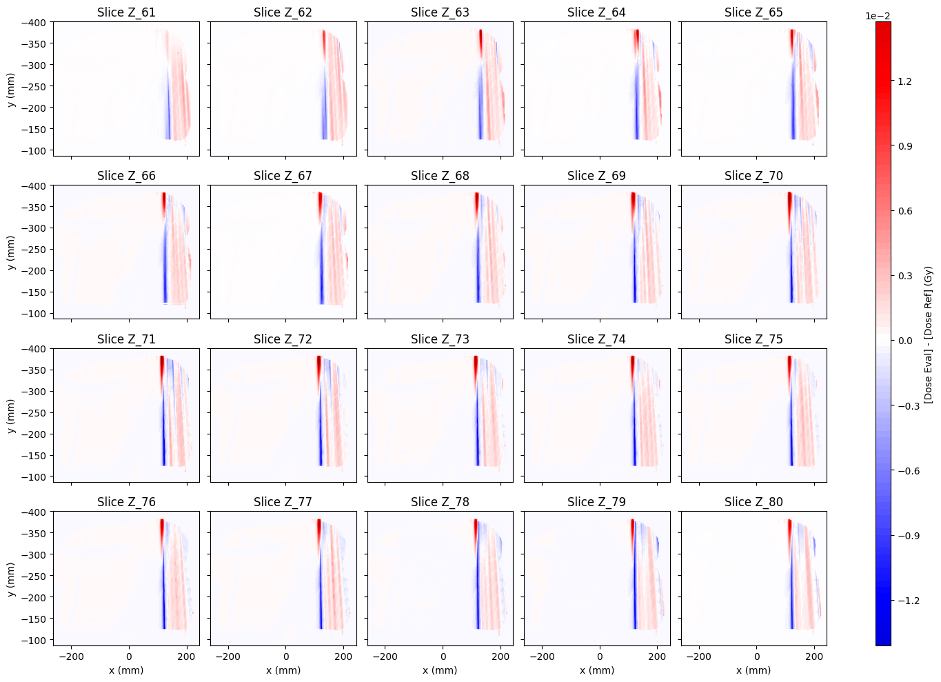
Let’ have a look at the dose distributions above and below the z-slice where they disagree the most

import matplotlib.pyplot as plt

dose_difference = dose_evaluation - dose_reference

max_diff = np.max(np.abs(dose_difference))

# get the z-slice with the maximum dose difference
z_max_diff, _, _ = np.unravel_index(np.argmax(np.abs(dose_difference), axis=None), dose_difference.shape)

# we consider 10 z-slices above and below the maximum dose difference
z_start = z_max_diff - 10
z_end = z_max_diff + 10

fig, axes = plt.subplots(figsize=(15,10), nrows=4, ncols=5, sharex=True, sharey=True)
ax = axes.ravel().tolist()
ax[0].invert_yaxis() # invert just once as y axes are shared

for i, dose_diff_slice in enumerate(dose_difference[z_start:z_end]):

    im = ax[i].contourf(x_ref, y_ref, dose_diff_slice, 100, cmap=plt.get_cmap("seismic"), vmin=-max_diff, vmax=max_diff)
    ax[i].set_title(f"Slice Z_{z_start + i}")
    
    if i >= 15:
        ax[i].set_xlabel("x (mm)")
    
    if i % 5 == 0:
        ax[i].set_ylabel("y (mm)")

fig.tight_layout()
cbar = fig.colorbar(im, ax=ax, label="[Dose Eval] - [Dose Ref] (Gy)", aspect=40)
cbar.formatter.set_powerlimits((0, 0))

plt.show()

As you can see, the largest dose differences are concentrated in small regions of the slices, which will end up in a fast gamma evaluation, as the computation will be immediate for those points where the dose difference is zero.

Now, we move to the actual calculation.

First of all, we define the acceptance criteria as 1% dose difference and 1mm distance

dose_percent_threshold = 1
distance_mm_threshold = 1

By default, the 1% of dose_percent_threshold refers to the 1% of the maximum value of the reference dose, i.e.

print(f"Maximum reference dose: {np.max(dose_reference): .2f} Gy")
print(f"Dose threshold: {np.max(dose_reference) * .01:.4f} Gy")

Maximum reference dose:  1.95 Gy
Dose threshold: 0.0195 Gy

In order to see in detail the messages traced by the PyMedPhys gamma, we import the logging module and set the logging level to DEBUG:

import logging
logger = logging.getLogger()
logger.setLevel(logging.DEBUG)

Now, we compute the gamma using the default settings of the PyMedPhys gamma, and measure its computation time with %%time

%%time

gamma = pymedphys.gamma(
    axes_reference, dose_reference, 
    axes_evaluation, dose_evaluation, 
    dose_percent_threshold, distance_mm_threshold)

INFO:root:Computing the gamma using global normalisation point

INFO:root:Global normalisation set to 1.946

INFO:root:Global dose threshold set to 0.019 (1.00% of normalisation)

INFO:root:Distance threshold set to [1]

INFO:root:Lower dose cutoff set to 0.389 (20.0% of normalisation)

DEBUG:root:Current distance: 0.00 mm | Number of reference points remaining: 106910

DEBUG:root:Points tested per reference point: 1 | RAM split count: 1

DEBUG:root:Current distance: 0.10 mm | Number of reference points remaining: 106910

DEBUG:root:Points tested per reference point: 23 | RAM split count: 1

DEBUG:root:Current distance: 0.20 mm | Number of reference points remaining: 28520

DEBUG:root:Points tested per reference point: 67 | RAM split count: 1

DEBUG:root:Current distance: 0.30 mm | Number of reference points remaining: 2888

DEBUG:root:Points tested per reference point: 135 | RAM split count: 1

DEBUG:root:Current distance: 0.40 mm | Number of reference points remaining: 602

DEBUG:root:Points tested per reference point: 227 | RAM split count: 1

DEBUG:root:Current distance: 0.50 mm | Number of reference points remaining: 128

DEBUG:root:Points tested per reference point: 348 | RAM split count: 1

INFO:root:Complete!

CPU times: user 2.17 s, sys: 549 ms, total: 2.72 s
Wall time: 2.61 s

Let’s breakdown the log trace of the gamma function:

1. Global normalisation set to 1.946: the global normalization is set by default to the maximum value of the reference dose

2. Global dose threshold set to 0.019 (1.00% of normalisation): the dose threshold value is (dose_percent_threshold * the global normalization / 100)

3. Distance threshold set to [1]: the distance_mm_threshold

4. Lower dose cutoff set to 0.389 (20.0% of normalisation): the gamma is computed only for those points where the dose value is bigger than this cutoff (20% of the maximum reference dose)

5. Current distance: 0.50 mm | Number of reference points remaining: 128:

   • Current distance: the current distance between reference grid point and evaluated grid points. The computation stops once a distance is reached for which the value of the gamma cannot improve further

   • Number of reference points remaining: the number of points left to be evaluated in the reference dose grid

6. Points tested per reference point: 348 | RAM split count: 1:

   • Points tested per reference point: the number of points considered in the evaluation dose grid for the current reference point

   • RAM split count: in case the number of points to check for the gamma value doesn’t fit into the designated RAM memory, the computation is split and performed in stages

The output stored in the gamma variable is a matrix containing the gamma index value for each point of the reference dose

np.shape(gamma)

(152, 158, 254)

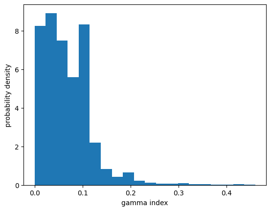
Let’s check the distribution of the gamma values to get a sense of the function output

import matplotlib.pyplot as plt

# remove NaN grid points that were not evaluated as the dose value was below the dose threshold
valid_gamma = gamma[~np.isnan(gamma)]

out = plt.hist(valid_gamma, bins=20, density=True)
plt.xlabel("gamma index")
_ = plt.ylabel("probability density")

Once the gamma index distribution has been computed, one can consider the gamma pass rate, defined as the fraction of points having $\gamma\le 1$, to assess the agreement between the reference and evaluated dose distributions.

Suppose that, for our purposes, we consider a gamma pass rate above 95% in order to have “passed” this comparison test.

Then, we check if the test passes (probably, you already guessed the answer by looking at the histogram above)

print(f"Pass rate(\u03B3<=1): {len(valid_gamma[valid_gamma <= 1]) / len(valid_gamma) * 100}%")

Pass rate(γ<=1): 100.0%

Indeed, all reference points have $\gamma\le 1$, thus the pass rate is 100%.

As expected, the computation of the gamma was quite fast because most of the grid points have zero dose difference

a = dose_difference[dose_difference == 0]
b = dose_difference[dose_difference != 0]

print(f"Fraction of grid points where [Dose Eval] = [Dose Ref]: {np.sum(dose_difference == 0) / len(dose_difference.flat) * 100:.1f}%")

Fraction of grid points where [Dose Eval] = [Dose Ref]: 39.5%

In practice, calculations of 3D gamma index distributions can be very time consuming. The problem is further exacerbated in applications where multiple comparisons are required.

For many applications, it is sufficient to simply calculate an accurate pass rate.

The PyMedPhys gamma function accepts optional parameters that can speed up the calculation in such cases:

• max_gamma: stop the calculation when a certain value of gamma is reached around the reference point

• random_subset: use only a random subset of the reference dose grid (range: 0-xyz)

Let’s see how these parameters affect the gamma calculation time.

For simplicity, we restrict ourself on the z-slice with the highest disagreement.

We also add a small shift to the evaluation dose distribution to obtain a worse gamma agreement which will make the computation slower:

# add 1% of the evaluation dose standard deviation where the evaluation dose in non zero
dose_evaluation_Z = np.where(
    dose_evaluation[z_max_diff] != 0,
    dose_evaluation[z_max_diff] + .1 * np.std(dose_evaluation[z_max_diff]),
    dose_evaluation[z_max_diff]
)
dose_reference_Z = np.array(dose_reference[z_max_diff])

# keep only the y, x axes
axes_reference_subset = axes_reference[1:]
axes_evaluation_subset = axes_evaluation[1:]

# increase the logging level to silence the traces of the PyMedPhys gamma
logger.setLevel(logging.ERROR)

Furthermore, let’s say we are now interested in evaluating all those points above 1% of the maximum value of the reference dose (instead of the default 20%): we pass the lower_percent_dose_cutoff to the PyMedPhys gamma function

%%time

gamma = pymedphys.gamma(
    axes_reference_subset, dose_reference_Z, 
    axes_evaluation_subset, dose_evaluation_Z, 
    dose_percent_threshold, distance_mm_threshold,
    lower_percent_dose_cutoff=1 # 1% lower threshold
    )

CPU times: user 653 ms, sys: 59.7 ms, total: 713 ms
Wall time: 712 ms

valid_gamma = gamma[~np.isnan(gamma)]

out = plt.hist(valid_gamma, bins=20, density=True)
plt.xlabel("gamma index")
plt.ylabel("probability density")
title = plt.title(f"Gamma passing rate: {np.sum(valid_gamma <= 1) / len(valid_gamma) * 100:.1f}%")

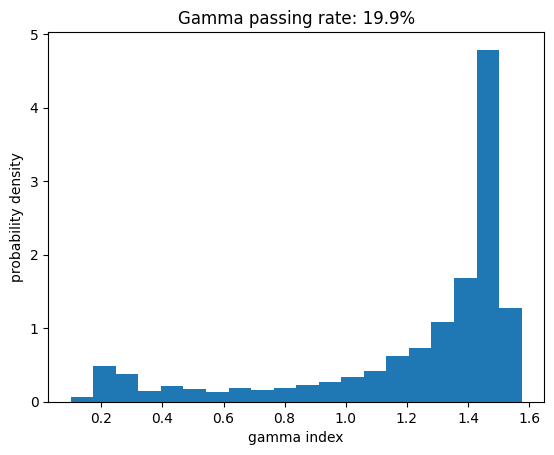
If we want to evaluate the gamma pass rate, we are uninterested in accurate gamma index values for $\gamma > 1$.

We can suppress calculations of gamma values above 1 by passing a suitable value (e.g., 1.1) to the max_gamma parameter of the PyMedPhys gamma function

%%time

gamma = pymedphys.gamma(
    axes_reference_subset, dose_reference_Z, 
    axes_evaluation_subset, dose_evaluation_Z, 
    dose_percent_threshold, distance_mm_threshold,
    lower_percent_dose_cutoff=1, # 1% lower threshold
    max_gamma=1.1 # stop when gamma > 1.1
    )

CPU times: user 438 ms, sys: 7.76 ms, total: 446 ms
Wall time: 446 ms

valid_gamma = gamma[~np.isnan(gamma)]

out = plt.hist(valid_gamma, bins=20, density=True)
plt.xlabel("gamma index")
plt.ylabel("probability density")
title = plt.title(f"Gamma passing rate: {np.sum(valid_gamma <= 1) / len(valid_gamma) * 100:.1f}%")

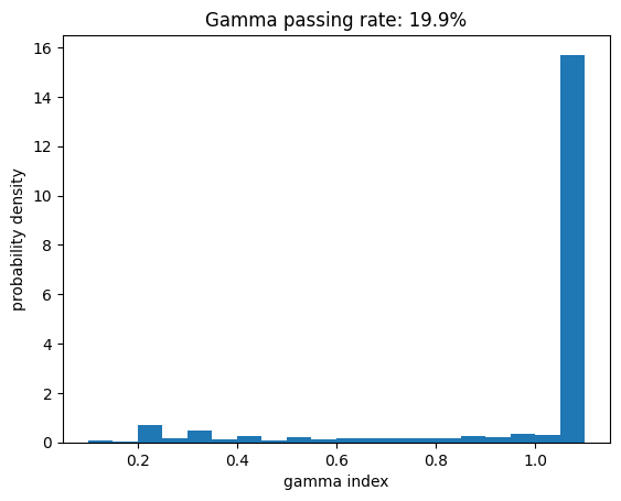
Notice how the gamma passing rate value (shown in the plot title) did not change. Of course now all the points with $\gamma > 1.1$ are collapsed to the 1.1 bin.

Finally, random sampling of a subset of the dose distributions for gamma index calculations may also produce a sufficiently accurate pass rate. This can also introduce significant decreases in calculation time.

We can compute the gamma index distribution from a random subset of grid points by providing a suitable fraction to the random_subset parameter of the PyMedPhys gamma function

%%time

gamma = pymedphys.gamma(
    axes_reference_subset, dose_reference_Z, 
    axes_evaluation_subset, dose_evaluation_Z, 
    dose_percent_threshold, distance_mm_threshold,
    lower_percent_dose_cutoff=1,
    random_subset=int(len(dose_reference_Z.flat) // 10) # sample only 1/10 of the grid points
    )

CPU times: user 487 ms, sys: 0 ns, total: 487 ms
Wall time: 487 ms

The $\gamma$ index distribution should look something like the following plot

valid_gamma = gamma[~np.isnan(gamma)]

out = plt.hist(valid_gamma, bins=20, density=True)
plt.xlabel("gamma index")
plt.ylabel("probability density")
title = plt.title(f"Gamma passing rate: {np.sum(valid_gamma <= 1) / len(valid_gamma) * 100:.1f}%")

As you can see, the computation time decreased and, despite the the PyMedPhys gamma function sampled one 10th of the points, the pass rate deviates by less than 1% from the true value. Therefore, you can use random_subset to get a sense of what could be the pass rate of the dose distributions you are assessing.

To conclude, you have performed several computations of the gamma index and the pass rate for 3D and 2D dose distributions using the PyMedPhys gamma.

Moreover, you have obtained fast pass rate computations by tweaking the max_gamma and random_subset parameters of the PyMedPhys gamma, independently.

Of course, both max_gamma and random_subset can be used at the same time. You are now ready to test them by yourself!