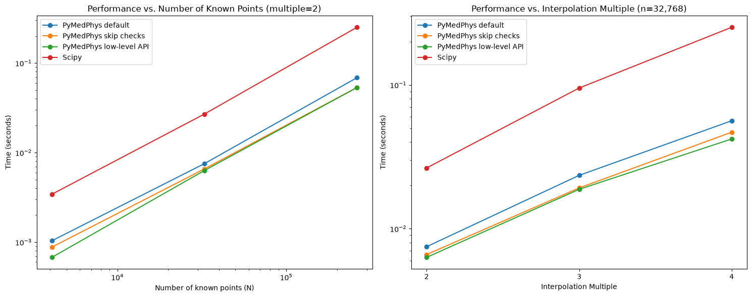
Multilinear Interpolation Comparison

This notebook compares PyMedPhys’ interpolation with SciPy’s RegularGridInterpolator, using reproducible inputs sized for a documentation build. To run it yourself, for example on Colab, install PyMedPhys first; the next cell does that and is skipped when the documentation is built.

Each implementation is warmed up before timing, so compilation is excluded, and its output is checked against SciPy. The timings include input checking and interpolator construction where applicable. The largest case below interpolates about two million points; increase the grid sizes for performance investigations on your own hardware. Numba uses at most two threads in this demonstration; adjust that limit along with the grid sizes when benchmarking larger workloads.

Imports

%pip install "pymedphys[user]"

import timeit
from typing import Sequence

from matplotlib import pyplot as plt
import numpy as np
import numba
import scipy

import pymedphys

# Keep the small demonstration from oversubscribing documentation build hosts.
numba.set_num_threads(min(2, numba.get_num_threads()))

def interp3d_scipy(axes, values, points_interp):
    interpolator = scipy.interpolate.RegularGridInterpolator(axes, values)
    return interpolator(points_interp)

def interp3d_pymedphys_skip_checks(axes, values, points_interp):
    return pymedphys.interpolate.interp(
        axes, values, points_interp=points_interp, skip_checks=True
    )

implementations = {
    "PyMedPhys default": pymedphys.interpolate.interp,
    "PyMedPhys skip checks": interp3d_pymedphys_skip_checks,
    "PyMedPhys low-level API": pymedphys.interpolate.interp_linear_3d,
    "Scipy": interp3d_scipy,
}


def benchmark(
    n_values: Sequence[int],
    interpolation_multiples: Sequence[int],
    fixed_n: int,
    fixed_multiple: int,
    implementations: dict,
):
    results = {
        "Performance with varying N": {
            "N values": n_values,
            "times": {name: [] for name in implementations.keys()},
            "fixed multiple": fixed_multiple,
        },
        "Performance with varying interpolation multiple": {
            "interpolation multiples": interpolation_multiples,
            "times": {name: [] for name in implementations.keys()},
            "fixed n": fixed_n,
        },
    }

    for n in n_values:
        run_combo(
            n, fixed_multiple, implementations, results["Performance with varying N"]
        )

    for multiple in interpolation_multiples:
        run_combo(
            fixed_n,
            multiple,
            implementations,
            results["Performance with varying interpolation multiple"],
        )

    return results


def run_combo(n, multiple, implementations, result):
    x = y = z = np.linspace(0, 1, n, dtype=np.float64)
    rng = np.random.default_rng(42)
    values = rng.random((n, n, n))

    xi = yi = zi = np.linspace(0, 1, n * multiple)
    points = np.column_stack(
        [mgrid.ravel() for mgrid in np.meshgrid(xi, yi, zi, indexing="ij")]
    )

    axes = (x, y, z)
    expected = interp3d_scipy(axes, values, points)

    for name, f_interp in implementations.items():
        # Warm up compiled functions and verify equivalent results before timing.
        actual = f_interp(axes, values, points_interp=points)
        np.testing.assert_allclose(actual, expected, rtol=1e-12, atol=1e-12)
        time = (
            timeit.timeit(
                lambda: f_interp(axes, values, points_interp=points),
                number=3,
            )
            / 3
        )
        result["times"][name].append(time)

def plot_results(results):
    _, (ax1, ax2) = plt.subplots(1, 2, figsize=(15, 6))

    # Left plot: Performance vs n for fixed multiple
    for name, times in results["Performance with varying N"]["times"].items():
        ax1.plot(
            np.array(results["Performance with varying N"]["N values"], dtype=np.int32)
            ** 3,
            np.array(times),
            label=name,
            marker="o",
        )

    ax1.set_xlabel("Number of known points (N)")
    ax1.set_ylabel("Time (seconds)")
    ax1.set_title(
        f"Performance vs. Number of Known Points (multiple={results['Performance with varying N']['fixed multiple']})"
    )
    ax1.legend()
    ax1.set_xscale("log")
    ax1.set_yscale("log")

    # Left plot: Performance vs n for fixed multiple
    for name, times in results["Performance with varying interpolation multiple"][
        "times"
    ].items():
        ax2.plot(
            np.array(
                results["Performance with varying interpolation multiple"][
                    "interpolation multiples"
                ],
                dtype=np.int32,
            ),
            np.array(times),
            label=name,
            marker="o",
        )

    ax2.set_xlabel("Interpolation Multiple")
    ax2.set_ylabel("Time (seconds)")
    ax2.set_title(
        f"Performance vs. Interpolation Multiple (n={results['Performance with varying interpolation multiple']['fixed n']**3:,})"
    )
    ax2.legend()
    plt.xticks(
        results["Performance with varying interpolation multiple"][
            "interpolation multiples"
        ]
    )
    ax2.set_yscale("log")

    plt.tight_layout()
    plt.show()

# Run the benchmark
n_values = [16, 32, 64]
interpolation_multiples = [2, 3, 4]
results = benchmark(
    n_values,
    interpolation_multiples,
    fixed_n=32,
    fixed_multiple=2,
    implementations=implementations,
)

# Plot the results
plot_results(results)