Gamma performance: a completed workstation audit

Recorded 27 September 2026; completed in 42 min 37 s. All 84 planned four-way comparison groups completed: 336 verified timed calls across 17 synthetic workloads, with a full warm-up before each timed call.

The results support a reduction in gamma runtime from PR #2066 and a substantial advantage for the PyMedPhys interpolation path on this workstation. They also show why a runtime prediction based only on the number of voxels can be wrong. These are synthetic computational experiments, including two volumes with the requested dose-grid dimensions and spacings. They do not establish performance on patient treatment plans.

Absolute waiting times for the larger volumes

The two volume examples use global 3% / 3 mm gamma, a 10% reference-dose cutoff, fixed 2 Gy normalisation and interp_fraction=10. Every eligible reference voxel is evaluated, without a random subset or early stopping on a pass. The “Two volume examples motivated by clinical workflows” section of the study guide describes the field construction and limitations.

Synthetic volume	Shape	Isotropic spacing	Total voxels	Above-cutoff voxels
SABR-like	201 × 241 × 241	1.25 mm	11,674,281	149,547 (1.28%)
Prostate and nodes	201 × 161 × 161	2.5 mm	5,210,121	245,100 (4.70%)

The SABR-like grid spans 250 × 300 × 300 mm between its outermost voxel centres; the prostate/nodal grid spans 500 × 400 × 400 mm. The latter has fewer total voxels but more above the cutoff, and takes longer. Both the dose distribution and the search needed to match it matter.

Median warmed time	Old PyMedPhys	New PyMedPhys	Old SciPy path	New SciPy path
SABR-like	3.99 s	3.17 s	12.57 s	12.89 s
Prostate and nodes	6.16 s	4.52 s	23.79 s	23.43 s

Each value is the median of four complete gamma calls. Times exclude imports, initial compilation, dose-array generation, full warm-ups and verification. Consequently, the elapsed time to run the audit is longer than the sum of these timings, and a first gamma call can take longer.

Here, speed ratio = PyMedPhys speed / SciPy speed = SciPy time / PyMedPhys time. Calculate this ratio within each matched round, then take its median:

Volume	Old source	New source	Observed new-source range
SABR-like	3.15×	4.07×	3.67–4.46×
Prostate and nodes	3.84×	5.15×	4.96–5.29×

These compare the two interpolation paths within a complete PyMedPhys gamma calculation, using one fixed SciPy package version. “Old/new SciPy” refers to the old/new gamma source using SciPy. Four Numba threads were used for the PyMedPhys path; this is the recorded configuration, not a thread-normalised kernel comparison. The ranges describe four observations, not confidence intervals.

How much improvement comes from this PR?

For the two volumes, the PR reduces the PyMedPhys path’s warmed time by 21.9% and 26.3%, respectively. Across all 17 workloads, the median reduction ranges from 13.0% to 31.4%. The 4–5× advantage over SciPy includes an advantage already present in the old code; it should not all be attributed to this PR.

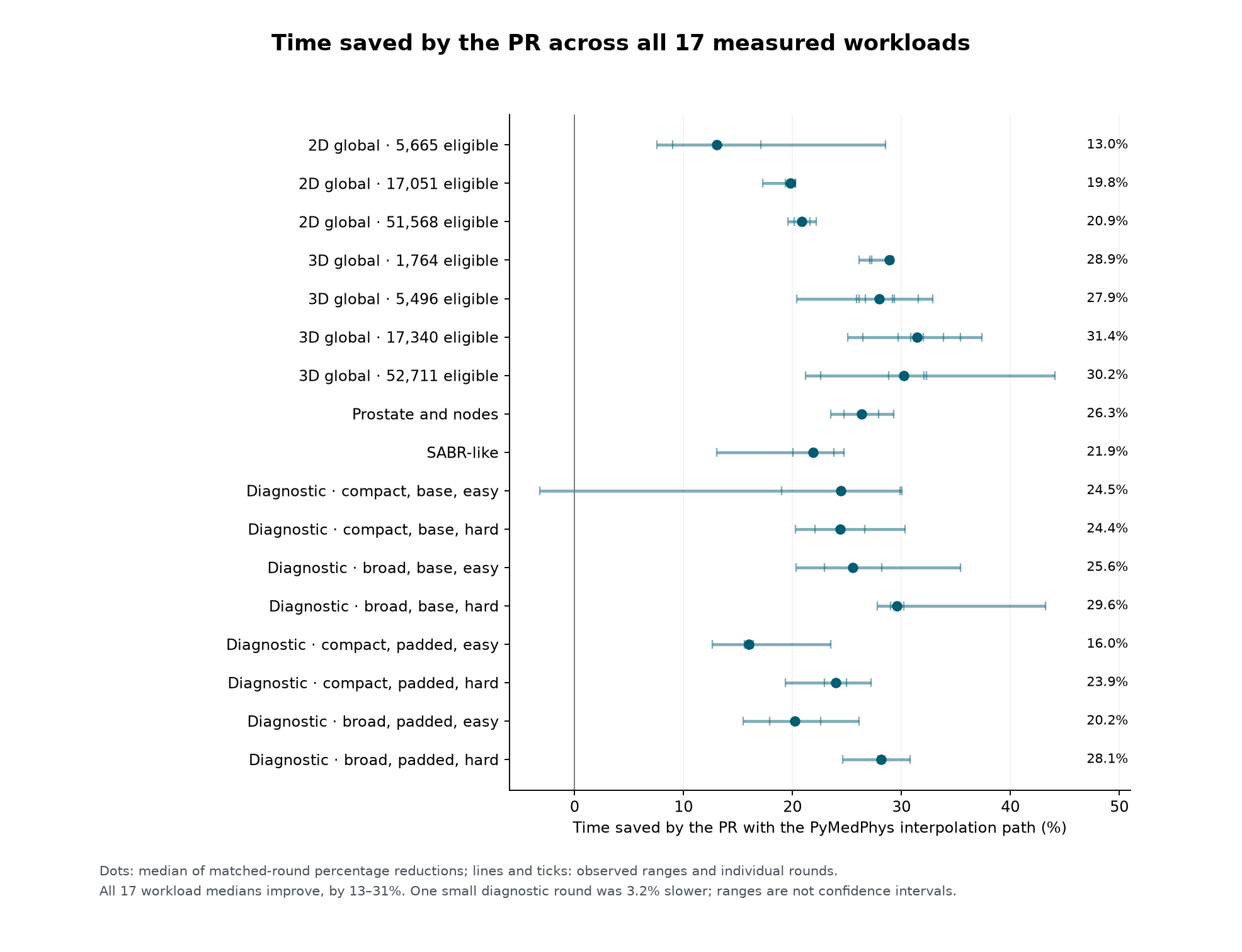
The plotted reduction is the median of 100 × (1 − new time / old time) within each round. This need not equal a percentage calculated from the two absolute medians in the table. Every workload median improved, although one round of a small diagnostic workload was 3.2% slower. SciPy-path changes were small and mixed; this audit does not establish a consistent SciPy-path gain.

A useful linear model within a specified workload

An eligible voxel is a reference voxel whose dose is at or above the cutoff. Let \(M\) be the number of eligible voxels divided by one million. Two simple models were fitted to the median time at each size:

• Proportional: \(t=bM\), with time \(t\) in seconds.

• With an offset: \(t=a+bM\), allowing a fixed setup cost \(a\).

Each size contributes one median to an ordinary least-squares fit in seconds. The plots use logarithmic axes to display the size range; the regression itself does not fit logarithms.

The 3D family has four sizes, 1,764–52,711 eligible voxels, with eight rounds per size. Its proportional slopes are:

Gamma path	Seconds per million eligible voxels	Exploratory 95% repeat interval
Old PyMedPhys	47.07	46.30–47.93
New PyMedPhys	32.80	32.22–35.50
Old SciPy path	191.17	187.70–207.84
New SciPy path	196.95	189.09–200.67

The new ratio of fitted slopes is 6.00×, with an exploratory repeat interval of 5.66–6.15×. This ratio of slopes differs from taking the median of paired speed ratios. For 2D, three sizes and four rounds give slopes of 4.25 and 7.51 s/million for new PyMedPhys and SciPy, a fitted ratio of 1.77×; no repeat interval is reported with only four rounds.

For the new 3D paths, including an offset gives \(t_{\mathrm{PyMedPhys}}=0.0351+31.93M\) and \(t_{\mathrm{SciPy}}=0.0722+195.16M\). Adding an offset does not automatically improve prediction. When one entire size is withheld from fitting, the maximum absolute prediction errors are:

New 3D path	Proportional model	Model with offset
PyMedPhys	18.0%	52.9%
SciPy	15.3%	2.7%

With only four sizes, these are useful stress tests, not comprehensive out-of-sample validation. The repeat intervals use 4,000 bootstrap samples of whole rounds, preserving pairing between sizes and variants. They describe repeat-timing uncertainty for these particular workloads, conditional on the rounds being exchangeable. They are not prediction intervals for another dose field or workstation. The new PyMedPhys slope was 6.8% lower in the later half of the session than the earlier half, so drift also limits this assumption. Its cause was not measured.

Does the model predict the separate volumes?

The two volume cases were excluded from fitting. Applying the small-grid proportional model overpredicts their runtimes substantially:

Volume	New PyMedPhys: predicted / measured	Overprediction	New SciPy: predicted / measured	Overprediction
SABR-like	4.91 / 3.17 s	55%	29.45 / 12.89 s	128%
Prostate and nodes	8.04 / 4.52 s	78%	48.27 / 23.43 s	106%

Both volumes also exceed the fitted eligible-count range. This therefore tests transfer to a different field and extrapolation together; the audit cannot separate their contributions. A precise fitted slope can still give an inaccurate prediction when the workload changes.

The earlier large-grid study found a new-source fitted ratio of about 5.24× over 60,101–6,149,042 eligible 3D voxels. There is no overlap with this audit’s core 3D eligible-count range. These studies have different sessions and coverage; the 5.66–6.15× interval above does not refine the uncertainty of the earlier 5.24× estimate. Their records and conclusions are kept separate.

Why voxel count alone cannot determine runtime

Eight diagnostic workloads vary field width, grid padding and dose mismatch. They use small, coarse grids to isolate computational effects, with global 3% / 3 mm gamma capped at 2. These grids are not clinical sampling recommendations.

Within each easy/harder pair, the reference dose, grid and eligible count are identical. The evaluation-dose displacement changes from (0.375, −0.5, 0.1875) mm to (4, −5, 2) mm, and its dose multiplier changes from 1.005 to 1.08. Both changes occur together, so their individual effects cannot be separated.

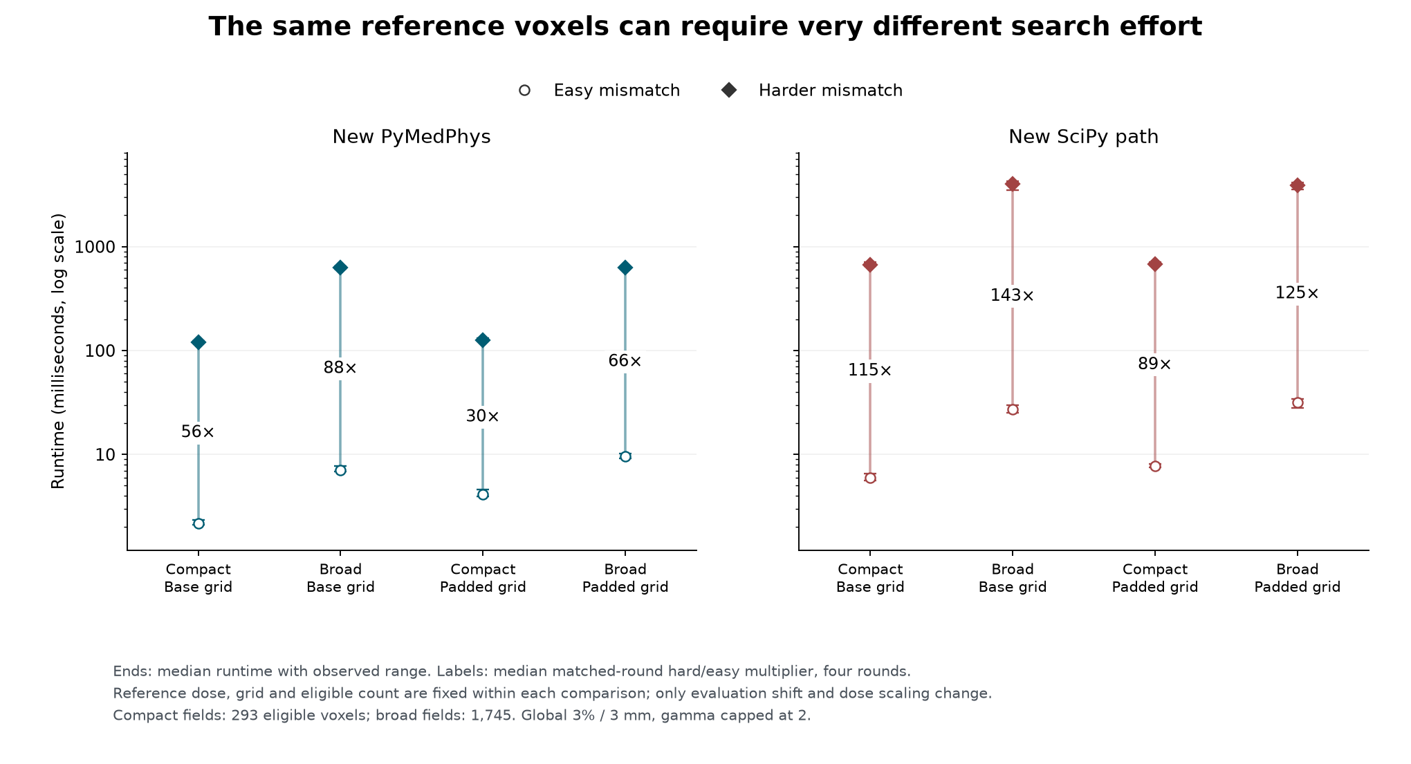
The harder mismatch takes 30–88× longer with new PyMedPhys, and 89–143× longer through new SciPy, using median matched-round multipliers. This is direct evidence that a fixed voxel count can require very different amounts of gamma search. The effect is large even though the harder cases still complete in seconds on these small grids.

In a separate comparison, padding increases the total grid from 20,181 to 68,479 voxels (3.39×) while preserving spacing, the existing dose samples and the eligible count. The added samples are below the cutoff.

For easy mismatches, padding increases new PyMedPhys time by about 35–90%. For harder mismatches, its median effect is about 0–4%. This is consistent with full-grid overhead being appreciable for very short calls, while search work dominates harder comparisons. The measurements do not uniquely identify each internal cost. Changing field width also changes its spatial distribution, so it is not a pure intervention on the eligible count.

A useful working explanation is:

\[ t \approx t_{\mathrm{setup}} + t_{\mathrm{grid}} + (\mathrm{cost\ per\ interpolation\ query}) (\mathrm{number\ of\ queries}). \]

Gamma searches progressively larger distances and removes resolved reference points from further searching. The required queries therefore depend on dose agreement, gradients, criteria and search settings as well as voxel count. Query counts were not measured here; they are a candidate explanatory variable for a future model, rather than a fitted result of this audit.

Coverage, numerical checks and provenance

The completed schedule contains 32 core 3D groups, 12 core 2D groups, 32 diagnostic groups and eight volume groups. Calibration is excluded from the 336 main timed observations. All planned main groups are present. This focused uncertainty audit does not include local gamma or every criterion covered by the separate coverage-oriented audit design.

The runner recorded exact old/new gamma-array equality for each interpolation path, and exact agreement between each timed result and its warm-up. The largest recorded PyMedPhys/SciPy absolute gamma difference was 2.59 × 10⁻¹⁴, with zero gamma pass/fail classification disagreements. These are numerical checks on the sampled synthetic workloads.

For publication, all 17 input sets were independently regenerated: dose-array hashes, total/eligible counts and gamma settings matched. The archived runner hashes and pinned source were checked, the saved model report was reproduced, and the fitted coefficients and paired ratios were independently recalculated. The original full gamma arrays were removed after the runner’s comparisons, and gamma was not rerun for this page, so the numerical findings above rely on the recorded full-array checks.

The comparison used old source 866f83edad85 and new source 9b3a8aa00b75. Hardware was an Intel Core Ultra 7 265HX, 20 logical CPUs, Windows 11 build 26200, Python 3.12.14, NumPy 1.26.4, SciPy 1.17.1 and Numba 0.67.0. Numba used four threads; OMP, OpenBLAS and MKL each used one. The gamma RAM chunk budget was 1.5 GiB, which is not a process-memory limit.

The same host and balanced within-round ordering reduce hardware and ordering confounds. CPU affinity, background load, power state and thermal conditions were not controlled or logged. This is one session on one workstation; repeat intervals do not establish cross-machine reproducibility.

Inspect or reproduce the evidence

• Raw checkpoint, gzip-compressed JSON and provenance.

• All timed observations, absolute summaries, paired speed ratios and PR time reductions.

• Model coefficients, complete model analysis and diagnostic paired effects.

SHA-256 of the uncompressed checkpoint: 42c959f1757d4bdd156f83ce77ac2414b7108a2b1f14c962090643f89673688e. The original upload’s SHA-256 is retained in the provenance file.

With the dependencies from the “Start” section of the study guide installed, rebuild these figures and tables from the repository root, without rerunning gamma:

python examples/gamma_uncertainty_evidence.py --input lib/pymedphys/docs/contrib/info/gamma-uncertainty-workstation/results.json.gz --output gamma-uncertainty-evidence-rebuilt

The generator verifies the pinned checkpoint and calculations. It leaves this authored explanation untouched. To collect a fresh audit on another workstation, follow the runtime-model uncertainty design in the two-hour workflow and retain its separate provenance and results.